Excel tips: how to dynamically highlight rows

Updated 5 April 2018

Question: Is it possible to dynamically highlight the current row in a table?

Answer: This question was posed by a retired accountant who uses Excel on a daily basis for community work. His eyesight isn’t what it used to be, and following the row across a wide screen proved a challenge.

The table in Figure 1 has 10 columns. Excel highlights the row number on the left of the screen but, as you scan across to the far right, it can be difficult to properly line up the correct row. Excel’s Conditional Formatting feature (Home ribbon) lets you conditionally change the format of a cell. We will use a formula to set the condition.

1. We will apply the conditional format to the whole table. To select the whole table, select a cell in the table and press Ctrl + a.

2. Click the large Conditional Formatting icon in the middle of the Home ribbon.

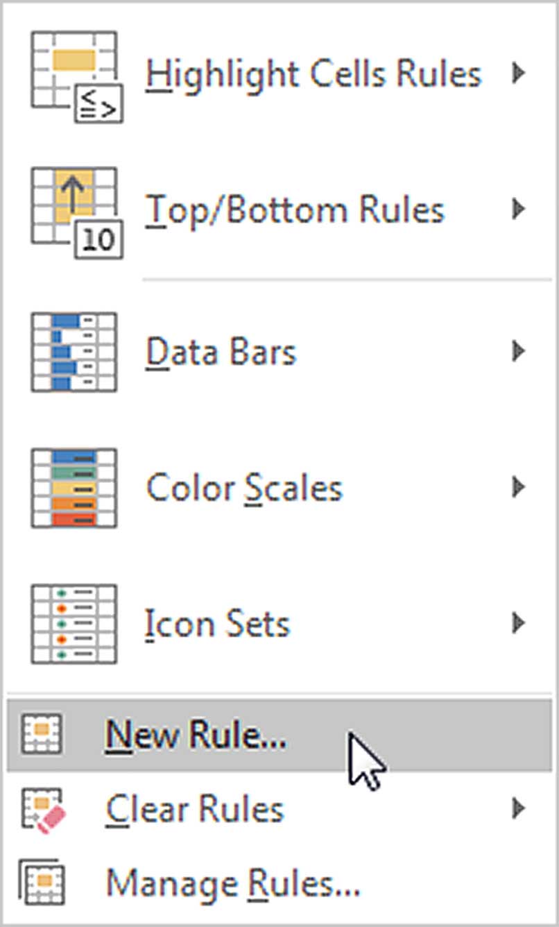
3. Select the New Rule option as per Figure 2.

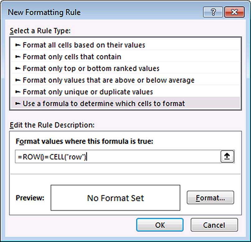
4. Select the last option in the top section “Use a formula … “ as shown in Figure 3.

5. In the rule box, enter the following formula as per Figure 3. 
> =ROW()=CELL("row")
(See the “Formula explanation” section on opposite page for more details.)

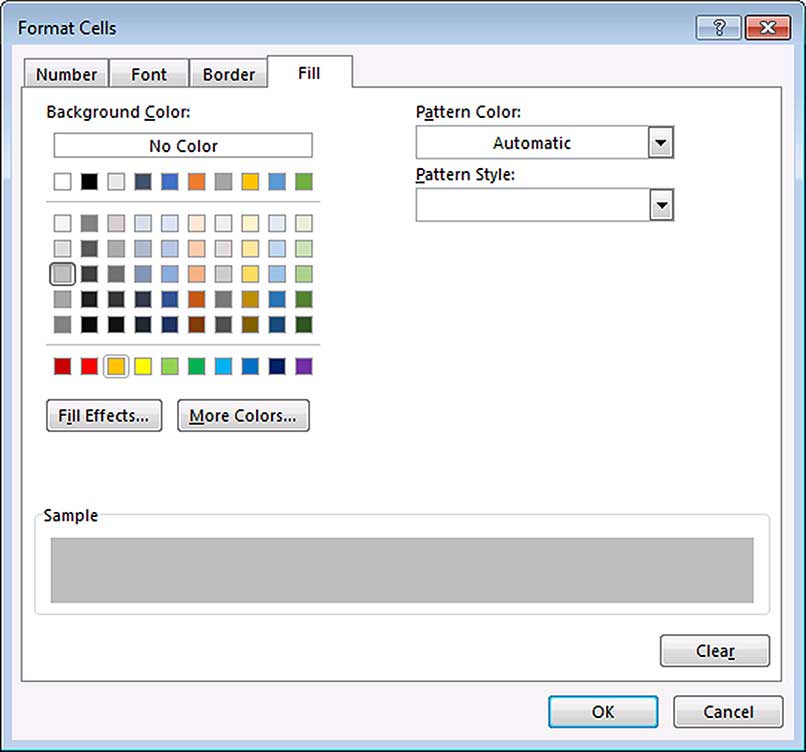
6. Click the Format button and use the Fill tab to choose a grey fill colour (or a brighter colour if you want it to stand out more) and click OK. See Figure 4. 

7. Click OK again to complete the conditional format. The whole row containing the cell you selected will be highlighted grey or the colour you chose.

If you select a cell in another row, the row colour won’t change. Selecting a new cell doesn’t cause Excel to re-calculate. The conditional format won’t update unless Excel re-calculates the formula. Pressing the F9 function key will force a calculation, which will update the format. We need a way to force the sheet to calculate each time we change the selected cell.

Event macros

Excel has a built-in macro feature called event macros that identifies certain actions. One of those actions is called a selection change. Excel monitors the sheet and triggers an event macro when the active cell changes. To create the event macro, follow these steps:

a) With the table sheet still selected, press Alt + F11. This opens a separate Visual Basic for Applications (VBA) window.

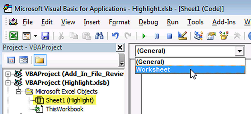
b) Click the sheet name involved on the left of the screen, as per Figure 5. The sheet name in the Figure 5 screen shot is Sheet1 (Highlight).

c) In the blank code window on the right, click the drop-down that displays General and choose Worksheet. See Figure 5.

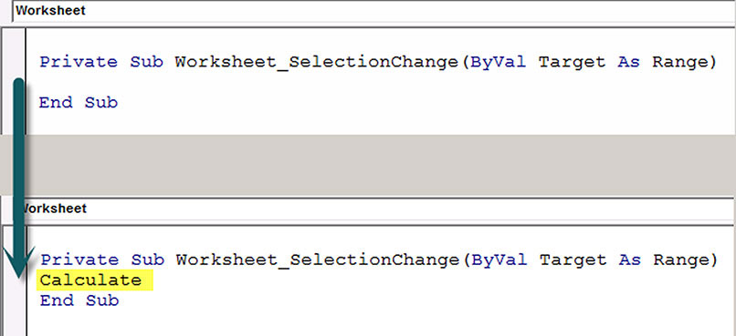
d) This will create a blank macro called Worksheet_SelectionChange. See top of Figure 6.

e) All we need to do is to type the word Calculate on the blank line, as shown on the bottom of Figure 6.

That’s it! Each time the selection is changed, the event macro forces Excel to calculate and the conditional format will automatically update.

=ROW()=CELL("row")

A conditional format formula must return TRUE when the format is to be applied and FALSE when it isn’t. You need to create a logical test statement, just like you use at the start of an IF function. 

The ROW function can be used in two ways. If you omit a cell reference, as per the formula shown above, it returns the row number of the cell it is used in. If you provide a cell reference, it will return the row number of that reference. For example, =ROW(A2) returns 2.

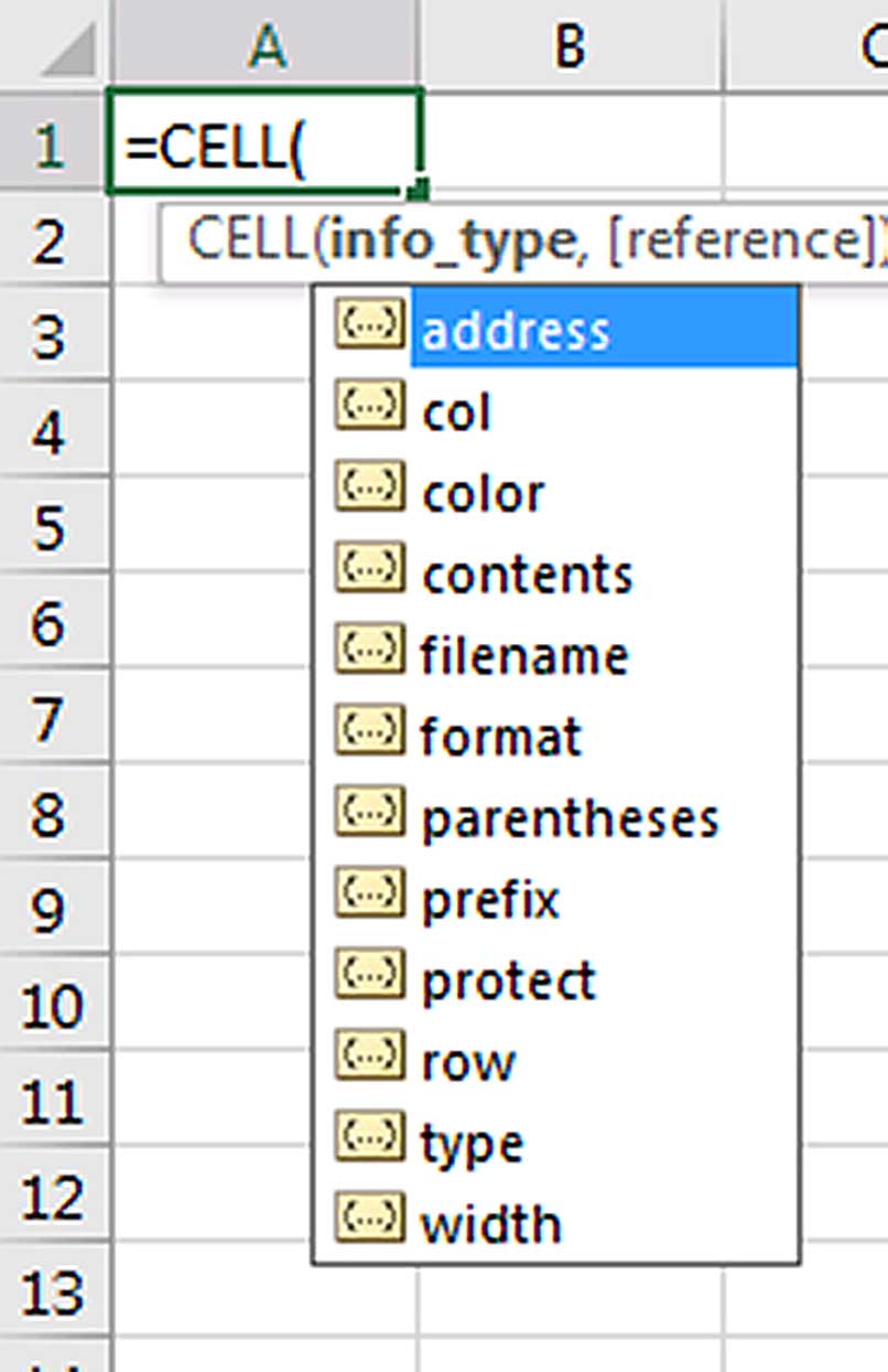
The CELL function is an information function. It doesn’t calculate anything; it returns information about whatever is selected. It takes two arguments, the first is the info_type, see Figure 7. The second is a Reference, which is optional. If you omit the Reference, then Excel returns the information based on the active cell. 

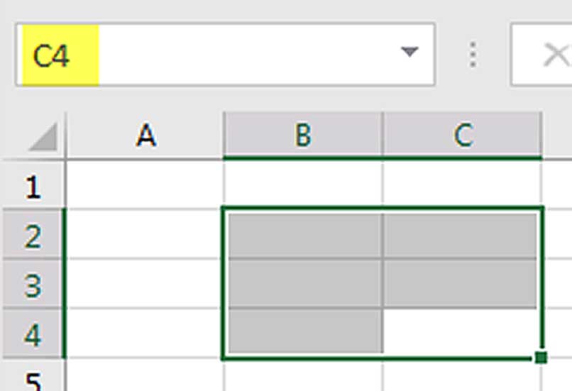
Every sheet has an active cell. Even if you select a range, one of the cells in that range will be the active cell. The Name Box (left of the Formula Bar) displays the active cell reference. In Figure 8, it displays cell C4. 

In the conditional format formula, I omitted the Reference from the CELL function, so the CELL function only returns the row number of the active cell.

It may seem like both functions are returning a row number. However, the ROW function returns a different number on each row of the table (cell C5 returns 5, cell B10 returns 10), whereas the CELL function is only returning a single number throughout the whole table range. The CELL function returns the row number of the active cell. When the two row numbers are equal, the grey format (or other colour) will be applied.

The file now contains a macro. When you try to save the file, a warning message will display as per Figure 9. Click No to this dialog.

There are two modern Excel file types that allow macros. They are Macro-Enabled files (.xlsm) and Binary files (.xlsb), see Figure 10.

If you have large files, the binary file type has some advantages. Its main disadvantage relates to its limited compatibility with non-Microsoft systems. If it doesn’t have to interact with non-Microsoft systems, then use the binary file type, otherwise use the macro-enabled file type. 

The companion video and Excel files (blank and complete) will go into more detail to demonstrate these techniques.

UPDATE

It was brought to my attention that the macro solution stopped the user from copying and pasting on the sheet. The solution was meant as an aid to improve visibility and navigation on a wide sheet and I didn’t consider copying and pasting.

After some investigation I have a partial solution that allows copying and pasting. There is still an issue that has a work around that is explained below.

Instead of the single word Calculate you need to insert an If statement as below

Private Sub Worksheet_SelectionChange(ByVal Target As Range)

If Application.CutCopyMode = 0 Then Calculate

End Sub

This checks the clipboard status and if something has been cut or copied the event macro won’t calculate. Remember Excel needs to calculate to update the conditional formatting.

To make this work effectively you need to copy (or cut), then navigate to the destination cell and press Enter. This is an old but little-known feature in Excel. When you press Enter you paste and clear the clipboard at once. This works perfectly with the above solution.

If you need to paste multiple times use Ctrl + v for each paste until the last paste and then use Enter. This also works perfectly with the solution.

Remaining Issue

A problem still arises when you only paste using Ctrl + v or right clicking. Moving the mouse or active cell will no longer update the row highlighting because the clipboard still has an entry (which stops the calculation). In this case pressing the Esc key clears the clipboard and everything starts working again.

Neale Blackwood CPA runs A4 Accounting, providing Excel training, webinars and consulting services to organisations around Australia. Questions can be sent to [email protected]