Loading component...
At a glance
I answered three Excel questions between May and July 2005.
1. I have an input spreadsheet that I distribute to users. I have used sheet protection to ensure users can only change input areas. The problem is users are still able to drag and drop within the input areas, which causes #REF! Errors. Is there a way to stop users dragging and dropping?
You can turn off the drag-and-drop feature in Excel by changing a setting. Unfortunately, that setting affects the whole of Excel. You can use an event macro to turn off drag-and-drop for a particular file. You can use an Event macro to change this setting. Event macros run when they are triggered. There are several triggers that Excel identifies that you can select to run macro.
The macros below will turn off the drag-and-drop feature when the file is activated and turn it on again when the file is deactivated.
Private Sub Workbook_Activate()
Application.CellDragAndDrop = False
End Sub
Private Sub Workbook_Deactivate()
Application.CellDragAndDrop = True
End Sub
When the first macro runs it stops the mouse arrow icon from appearing when you point to the border of a cell.
Installation
Since these are Event macros they must be installed differently to standard macros.
Press Alt + F11, this opens the Visual Basic for Applications (VBA) Window. On the left of the screen open the file so you can see the sheets listed – see Figure 1.

Double click the ThisWorkbook item at the bottom of the Microsoft Excel Objects list.
Copy the macros from above and paste them into the code window on the right of the VBA window. That’s it, the macros are ready to run.
These macros run automatically when the file is activated or deactivated. You deactivate a file by accessing another file. Open a new blank Excel file. Change back to the original file and you won’t be able to use the drag and drop feature.
These macros do not stop the user from using cut and paste. Cut and paste can also cause #REF! errors in Excel. Turning off cut and paste is more complex than turning off drag-and-drop.
File types
Back in 2005 Excel only had one file type .xls. With the release of Excel 2007 there were three new file types created. The standard Excel file type now is .xlsx and this does not allow macros. The other two file types can contain macros.
If you install the above code in a standard Excel file when you try to save the file a warning message will pop up – see Figure 2.

This is a warning that the standard Excel file type does not support macros. Make sure you click the No button. If you click Yes, you will lose the macros. When you click No, you will see the Save As dialog.
Use the Save as type drop down to select either a Macro-Enabled Workbook file type .xlsm or an Excel Binary Workbook .xlsb. See Figure 3.
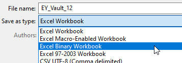
Note: You will need to make sure macros are enabled for this technique to work.
2. I've seen spreadsheets with shading on every second row. Is there an easy way to do this, other than manually formatting the rows?
Since Excel 2007, the Format as Table feature on the Home ribbon has included alternating row shading as a default for Excel tables. If you want to mimic that shading in a normal range, you can use a conditional format. Follow these steps to apply the format.
i. Select the range you want to format.
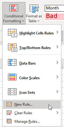
ii. On the Home ribbon click the Conditional Formatting icon drop down and choose New Rule – see Figure 4.
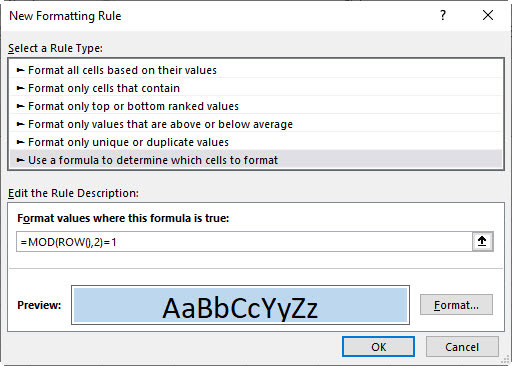
iii. In the top section select the last option “Use a formula to …”. In the formula box in the bottom section, enter this formula – see Figure 5.
=MOD(ROW(),2)=1
I will explain this formula after the instructions.
iv. Click the Format button, click the Fill tab, choose a colour, and click OK.
v. The completed dialog is shown in Figure 5.
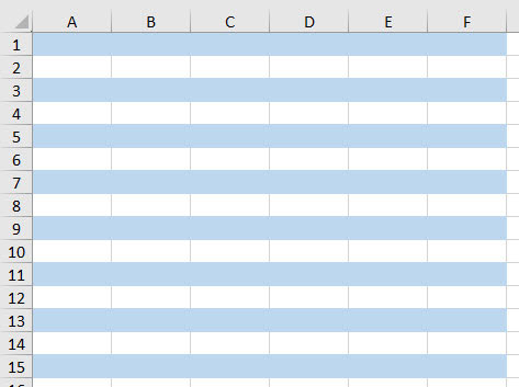
vi. Click OK to apply the format. See the result in Figure 6.
Formula explanation
When creating a formula for a conditional format, the formula must return TRUE for the format to be applied. This formula includes two functions.
The ROW function returns the ROW number. When no reference is supplied between the parentheses, the ROW function returns the row number of the current row.
The MOD function returns the remainder after dividing one number by another number.
The ROW function provides the ROW number for each row in our selection. The MOD function divides the row number by two. This means every second row is going to have a remainder of one.
Since we are comparing the MOD result with one, only the odd numbered rows will be formatted with the colour. If you wanted only the even row numbers to be coloured, you would compare the MOD result with zero.
3. I have three cells with three parts of a heading. I want to combine the three parts and display each part in a single line in a single cell as three lines in a single cell. You achieve the same effect by using Alt + Enter where using data entry in a cell. Can this be done with a formula?
Yes, formulas can insert a line break within a cell. There are a couple of solutions to this problem. The solution you use will depend upon the Excel version that you have.
All versions
Excel has a function called CHAR that allows you to insert special characters within your formulas. Using the number 10 between the parentheses of the CHAR function will return the line break character.
If we assume that the three cells that we want to combine are A1, A2 and A3, then the following formula will create a single heading with three separate lines.
=A1&CHAR(10)&A2&CHAR(10)&A3
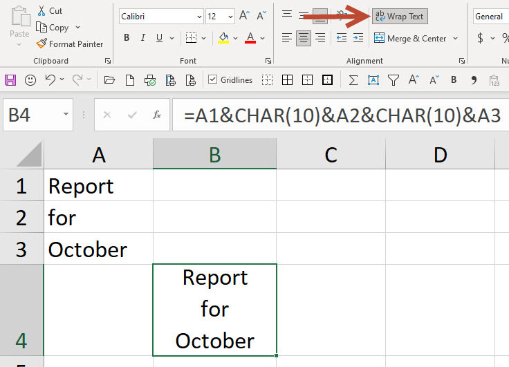
You need to apply the Wrap Text format to the cell to see the three separate lines – see Figure 7.
This solution is not scalable. You need to refer to each individual cell in the formula. If you have the subscription version of Excel, you have another option.
Microsoft 365 (subscription version)
In the latest version of Excel, you have access to the TEXTJOIN function. This provides a scalable way to build text strings based on a range of cells. The formula that works in the subscription version is.
=TEXTJOIN(CHAR(10),1,A1:A3)
In the TEXTJOIN function, you must first specify what is called the delimiter. A delimiter is a character that you wish to place between the entries from the range. The 1 in the middle of the function instructs Excel to ignore blank cells within the range. On the end of the function, you refer to the range that you want to combine. You also need to apply the Wrap Text format to the cell for this technique to work correctly.
The result is shown in Figure 8.
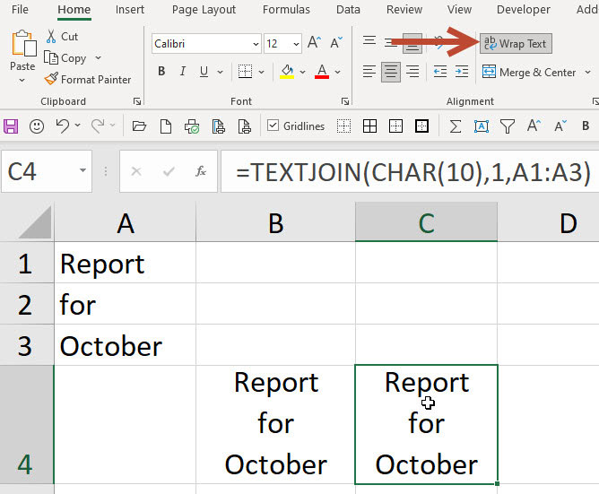
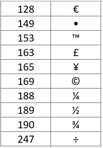
Figure 9 shows other characters and their respective numbers that you can access via the CHAR function.
The companion video and Excel files (Blank and Complete) will go into more detail to demonstrate these techniques.
Neale Blackwood CPA runs A4 Accounting, providing Excel training, webinars and consulting services. Questions can be sent to [email protected]

