Use Excel relationships to enable PivotTables to report by financial year

Question

Is it possible for PivotTables to work with our financial year, rather than the calendar year?

Answer

The easiest way to work with our financial year is to use a date table. This solution applies to Excel 2013 and later versions. You can apply this solution to Excel 2010 if you install the free PowerPivot add-in, as discussed in my August 2016 article, but Excel 2010 has different instructions to achieve the same result. 

The Data Model in modern Excel allows you to create a relationship between tables, just like a relational database. There is a Relationships option in the Data ribbon, which I featured in my October 2015 article. You can create your own date table in Excel and relate it to any other data source that contains dates.

Efficiency

In the past, the typical method of handling financial years involved adding extra columns to your data that included financial year calculations. The problem with this method is the increase in file size. If your transactional data is 100,000 rows long and you add five columns for financial year calculations, then you have added half a million formula cells to your model.

A date table covering three years would have about 5500 formulas to achieve the same result. A standard date table might look like the one in Figure 1. The formulas for these columns appear later in the article. While I don’t have room here to explain all the formulas, I cover them in more depth in the companion video.

Requirements

1. Use a standard date – no fractions (times). 
2. Ensure there is a row for every single day of the year – no gaps or duplications.
3. Start the date table with the earliest date from your data set.
4. Include at least another year’s worth of dates after the last date in the data set. Include a six-monthly task to regularly expand those future dates so you can keep ahead of yourself.
5. Add as many columns as you need to analyse your daily results. 

Data set dates

This solution assumes the date column in your data set has no time fraction. Many systems include a time stamp in their date fields. This will impact the usefulness of this date table technique. If there is a time, it must be removed. You can use the TRUNC function to remove times from a date.

Column headings

I use the following abbreviations in the column headings: Mth for month; Num for number; and Fin for financial. Feel free to use the whole word.

Format as Table (Home ribbon tab)

I have applied the Format as Table option to define the table in Figure 1. This feature has many advantages. Its main advantage is automatically expanding the table to include new rows and columns. This feature also automatically copies formulas to new rows. I have named this table tblDates. I use the tbl prefix as a naming convention for tables.

When you select a cell in a Formatted Table, the Design ribbon displays. You can rename the table in a box on the far left of the Design ribbon tab. In the same file, I have also used Format As Table on a daily sales table and named it tblSales.

Refreshing PivotTables

If the PivotTable data source changes or expands, as mentioned above, you must refresh the PivotTable to show the updates. The keyboard shortcut to refresh is Alt + F5. You must select a cell in the PivotTable to use it.

The formulas in the table below relate to Figure 1.

Heading Cell Formula

FinYear B2 =YEAR(A2)+IF(MONTH(A2)>6,1,0)
FinYearMthNum C2 =MONTH(A2)+IF(MONTH(A2)>6,-6,6)
FinYear MthNumName D2 =TEXT(C2,"00")&"_"&TEXT(A2,"mmm")
FinYearQtr E2 ="Q"&ROUNDUP(C2/3,0)
FinYearHalf F2 =IF(C2<=6,"H1","H2")

Formula note

I created the above formulas before applying the Format as Table option. If you use Format as Table first, then the formulas may use structured table references, which are like range names. This is demonstrated in the companion video.

Creating a Relationship

I covered these steps in more detail in the October 2015 article. Note: the Relationship icon will only be available if you have two or more Formatted Tables in a file.

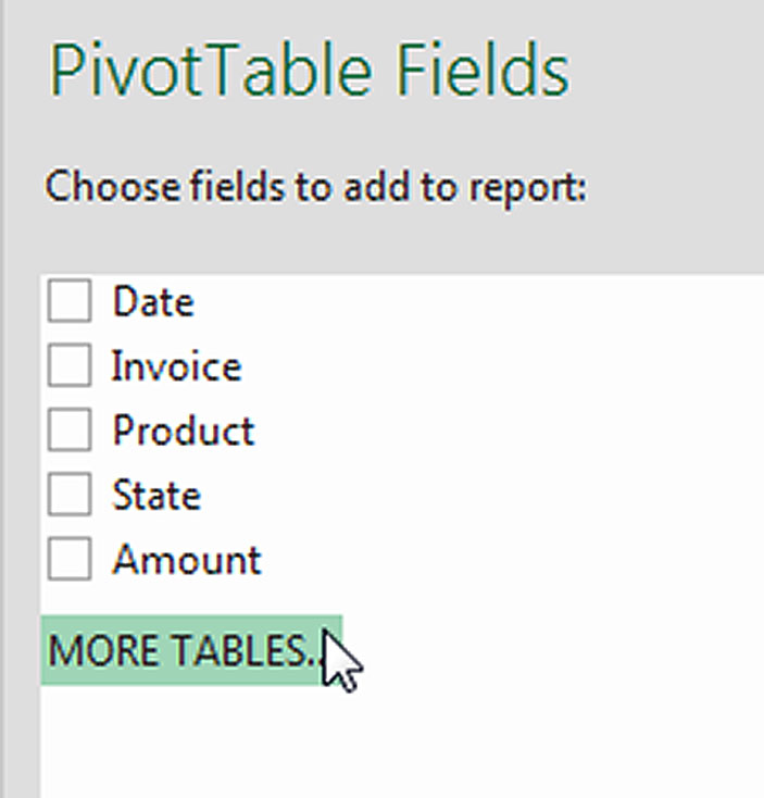
Click the Data ribbon, then click the Relationships icon (right side of ribbon). Click the New button. Make the selections as shown in Figure 2. Click OK and then click Close. Select a cell in the sales table and press the following keys in sequence Alt n v Enter. This shortcut inserts a blank PivotTable in a new sheet using the current table as the data source. Click the More Tables option – see Figure 3.

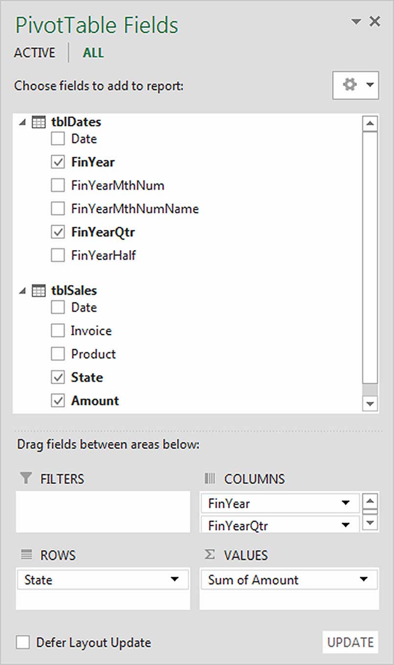
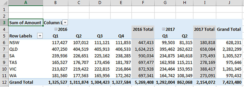
A dialog opens asking you if you want to use the Data Model. Click Yes. This will create another new PivotTable and gives you access to all the fields in both related tables. Figure 4 shows the fields selected and Figure 5 displays the resulting PivotTable report.

Optional columns

If you need to analyse daily sales in more depth, you can add more columns to your date table to allow this analysis. For example, you may want to classify each date by its day of the week. You could also classify dates as a workday, weekend or public holiday. Consider other daily metrics, such as temperature or rainfall, that may affect sales.

The companion video and an Excel file may assist your understanding.

Neale Blackwood CPA runs A4 Accounting, providing Excel training, webinars and consulting services to organisations around Australia. Questions can be sent to [email protected]