Excel tips: how to use Flash Fill and Formula Auditing

I answered four questions in February and March 2004.

1. Is there a way to list all the range names in a workbook?

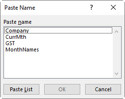
Yes, this is a useful technique for documenting the file. Select a blank cell with no entries below it or in the column on the right. Press the F3 function key and then click the Paste List button – see Figure 1.

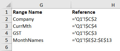
A list of all the range names, plus their references will be pasted as per Figure 2.

I added the headings in row 1. Cell G2 was selected when I clicked Paste List.

This list is not dynamic. If you add or delete a range name you need to redo the Paste List operation.

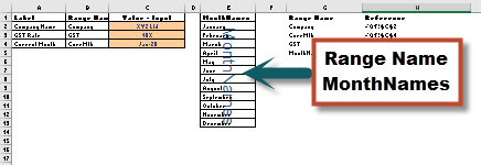
Another way to see where the names are on a specific sheet is to reduce the zoom percentage below 40% (Figure 3). This will display some of the range names in-situ on the sheet. 

Note: you can hold the Ctrl key down while moving the mouse scroll wheel to quickly zoom in and out of a sheet. This shortcut works on most systems including internet browsers.

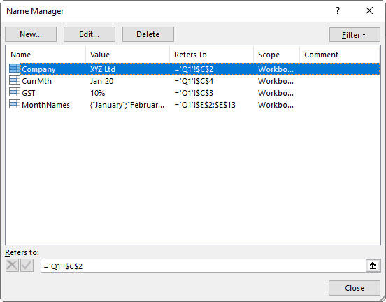
On the Formulas ribbon tab the Name Manager allows you to see all the names and their references (Figure 4), plus you can create new names, edit and delete names. You can sort by the various columns by clicking on the headings in the Name Manager list.

You can also press Ctrl + F3 to display the Name Manager. The F3 function key is dedicated to range names. The columns can be rearranged by clicking, holding and dragging the headings row with your mouse.

You can add Comments to range names when you create them with the New Name dialog or by using the Edit button in the Name Manager dialog. Comments can be added as part of your documentation of the range names. Comments can be used to explain range name use.

Name Box

Another way to see a list of range names is to use the Name Box. This is to the left of the Formula Bar and above the column letters. It normally shows the current cell reference. Clicking the drop down shows a list of range names. Clicking a name will take you to the name.

2. Have you got any tips to debug a formula that is displaying an error?

On the Formulas ribbon tab there is a Formula Auditing section where you can analyse formulas – as shown in Figure 5. 

You can trace precedent and dependent cells/ranges.

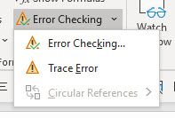
You can use the Error Checking drop down to trace errors. See Figure 6.

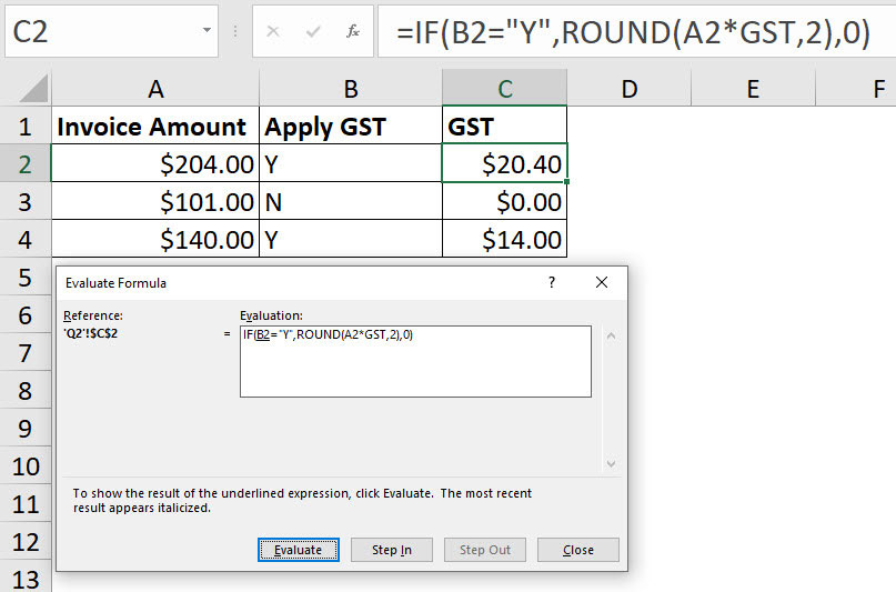
You can use Evaluate Formula to step through the various parts of the formula – see Figure 7 for an example.

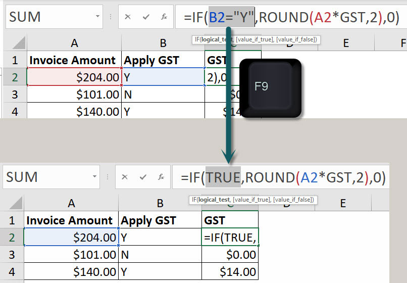
You can also calculate part of a formula in the Formula Bar by selecting it and pressing the F9 function key – see Figure 8. 

You must select a part of the formula that can be independently calculated for this technique to work. After using this technique always press the Esc key, otherwise the result will remain typed into the formula. You can also use Undo if you inadvertently accept the change.

3. I have a column with names in the format John, Smith. I need to split them into first name and last name.

You have at least three options.

Formulas

A formula can do the split. If the name was in A2 then this formula will extract the first names.

=LEFT(A2,SEARCH(",",A2)-1)

The LEFT function extracts characters from the left of the cell. The SEARCH function returns a number representing the position of the character being searched for within the cell. We deduct 1 from the SEARCH result to ensure the comma is not displayed.

This formula will extract the second name.

=RIGHT(A2,LEN(A2)-SEARCH(",",A2)-1)

The RIGHT function extracts characters from the right of a cell. The LEN function calculates the total number of characters in a cell. Spaces are counted as characters. To avoid including the space we deduct 1 from the result of the LEN function minus the SEARCH function.  

If you also have middle names the formulas become more complex. 

Text to Columns

Another technique is to use the Text to Columns option in the Data ribbon tab. This requires that the columns to the right of the column being split are empty. I will copy the range to the right – this will leave the original list unchanged. Select the new range, click the Data ribbon tab and click the Text to Columns icon.

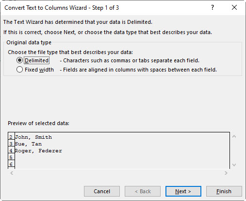
Ensure the Delimited option is selected and click the Next button as per Figure 10.

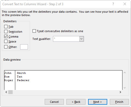
Select the Comma option and click Finish. See Figure 11.

Monitor the Data preview window at the bottom of the dialog as it displays what the output will look like.

You can use Undo to revert the data back to the original layout if it doesn’t work as you expect. 

You will need to use the TRIM function (see Formulas solution above) to remove the leading space from the last name. You could then use Paste Special Values to paste the amended last names on top of the list with spaces.  

If the names themselves don’t contain any spaces, you could select both the comma and space delimiters in Figure 11. Make sure the “Treat consecutive delimiters as one” box is ticked. This would remove the leading space from the last name. 

If you are doing multiple conversions, the dialog will retain the settings you last used.

Flash Fill

This sounds like a super hero and it does perform some superhuman tasks.

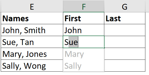
Enter two labels in the heading row, for example, First and Last as per Figure 12. The technique requires a table layout to work.

In cell F2 type John. In cell F3 type S – see Figure 12 for what Excel does – it’s like magic. 

Press Enter to accept all the entries. This will also work on a long list.

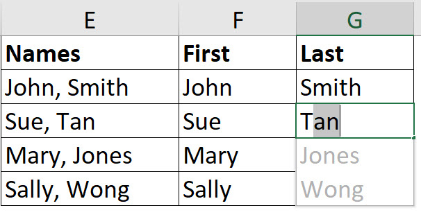
In cell G2 enter Smith. In cell G3 start to type T – see Figure 13.

You can force Excel to apply Flash Fill by selecting the range with the example cells plus the blank cells and pressing Ctrl + E. Flash Fill uses pattern recognition to create the entries. You can train it by including more examples.

Power Query could also do the split. If you are doing this regularly, using Power Query could automate the process. Not all versions of Excel have Power Query built in. Power Query is built in to Excel 2016 and later versions. It is a free Microsoft add-in to Excel 2010 and 2013.

4. I have a column of figures that have a leading apostrophe (‘). Excel treats them as text. How can I convert them to numbers that Excel will use?

There are a few ways to achieve this.

Built-in “Numbers Stored as Text” error

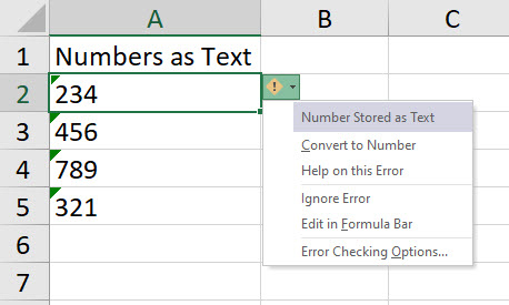
Excel identifies cells that have numbers that are stored as text – see the small green triangles top left of the cell in Figure 14. 

This can happen when numbers are imported from other systems. Numbers stored as text will be ignored in calculations and have been the source of many errors in Excel over the years.

In addition to identifying the numbers as text, Excel has the ability to convert them into real numbers.

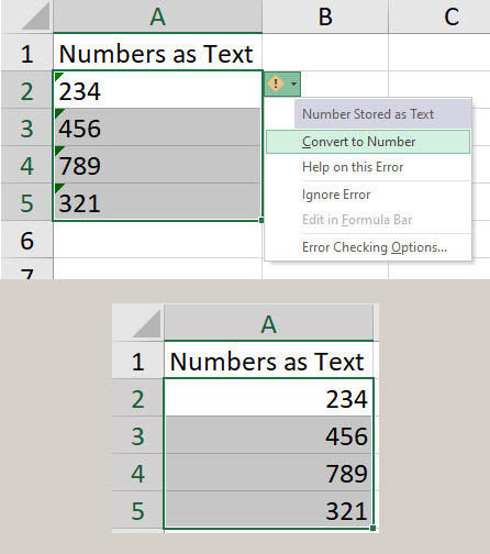
Click the error icon drop-down (Exclamation mark) – see Figure 15.

Click the Convert to Number option to fix the error.

This works if all the entries in the range are affected. If only some are affected, the next method is a more reliable solution.

Use Paste Special

Another technique involves the Paste Special dialog. In a blank cell enter a 1. Copy that cell. Now select the range that has the numbers as text and right-click the range and choose Paste Special.

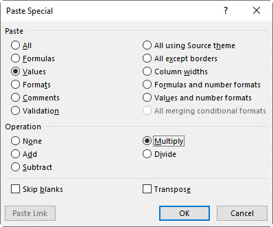
In the Paste Special dialog choose Values in the top section and Multiply in the middle section – see Figure 16. 

Click OK. Job done. 

You use Values in the top section to ensure you don’t paste or remove any formats when you do the paste.

This technique can also be used to convert negative numbers to positives. Simply type -1 in the cell and copy it and follow the same steps.  

Use a formula

You can also place a formula in a column next to the problematic range. If the first cell with a text number is A2, then this formula will convert it into a real number.

=A2*1

You can copy this down and then use Copy and Paste Values to paste the results on top of the original column and then remove or clear the formula column.