Excel tips: how to troubleshoot the #N/A error

Question

The IFERROR function handles all Excel formula errors the same. Is it possible to handle the #N/A error differently?

Answer

There are three popular functions that can return the #N/A error: VLOOKUP, HLOOKUP or MATCH. The #N/A error means that the code or item being looked up, or searched for, is not in or within the range involved. 

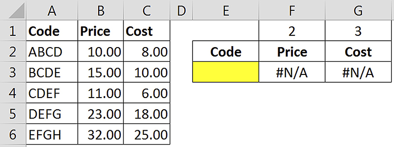
The formula examples below will use the table and layout in Figure 1. Cell E3 is for input.

TI will use the VLOOKUP function as an example. The formula in cell F3 is:

=VLOOKUP($E$3,$A$2:$C$6,F1,0)

This has been copied to cell G3.

VLOOKUP notes

There are two things to note about the above VLOOKUP function.

The reference to cell F1. Cell F1 is what I call a helper cell. Helper cells make the final formula easier to copy across. Often, users will key in 2 instead of linking to a cell that contains 2. The 2 represents the second column in the table. When you key in 2, you must edit the formula after you copy it across so that it refers to other columns in the table.

Linking to a helper cell makes it easier to copy the formula across and extract data from other columns.

An alternative could be to use a MATCH function to provide a flexible column reference.

The use of ,0 at the end of the function. This is instead of ,FALSE and specifies an “exact match” lookup. This means the code to lookup must be in the leftmost column of the table. In Excel, FALSE and 0 (zero) are the same, so it is easier to use ,0 at the end of the VLOOKUP than ,FALSE. One common reason for the #N/A error is that the cell that contains the value to lookup is empty.

This is the case in Figure 1. To avoid an error due to a blank cell, you can use the following formula:

=IF($E$3="",0,VLOOKUP($E$3,$A$2:$C$6,F1,0))

The IF function ensures a zero is displayed if cell E3 is empty. Using two quotation marks together "" is the easy way to test for a blank, or empty, cell. Once you have dealt with the blank cell issue, you now need to find out if an incorrect code has been entered.

An #N/A due to an incorrect code can mean a few things.

1. A data entry error – user will need to re-enter the correct code.
2. The code entered is new – the new code needs to be added to 
3. the table.
4. The table needs to be re-sorted – applies only to "approximate match" lookups discussed below.

The first issue type is the most common and we can return a more descriptive error message than #N/A. The other two errors relate to the data table. If a new code needs to be added, that may be done by the user or the file owner. Either way, the table needs to be updated before the user can move on.

Approximate match lookup

The third error relates to an option in the lookup functions themselves. If you omit the ,0 or ,FALSE from the end of the VLOOKUP, then the default setting is used. The default is an "approximate match". This means the table used in the VLOOKUP function must be sorted in ascending order by the leftmost column in the table.

Excel 2013 added a new function to handle #N/A errors more easily. The new function is IFNA. This function allows you to handle the #N/A error differently to other errors. In previous versions, a much longer formula was required to handle #N/A differently.

Excel 2013 formula for cell F3

=IFNA(IF($E$3="",0,VLOOKUP($E$3,$A$2:$C$6,F1,0)),"Code not in table")

Excel 2010 and earlier versions formula for cell F3

=IF($E$3="",0,IF(ISNA(VLOOKUP($E$3,$A$2:$C$6,F1,0)),"Code not in table",VLOOKUP($E$3,$A$2:$C$6,F1,0)))

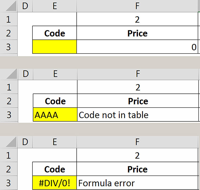
The IFNA function only has two arguments separated by a comma. The formula to review is the first. The second is what to do if the #N/A error is returned by the formula under review. You can display text, as shown above, or a number, e.g. zero, or another calculation. The above formulas will display a zero if cell E3 is blank and will display the text “Code not in table” if the entry in cell E3 is incorrect. This applies to the “exact match” errors mentioned in issues 1 and 2 above.

One more error issue

The last type of error you need to be aware of is if the cell to lookup (E3 in our examples) contains an error. In our previous example, that is unlikely as the cell is an input cell, but many times the lookup cell is itself a formula. If that formula returns an error, you also need to handle that. We need to add the IFERROR function to the above two formulas to handle all other errors. The IFERROR function was added in Excel 2007.

Excel 2013 formula for cell F3

=IFERROR(IFNA(IF($E$3="",0,VLOOKUP($E$3,$A$2:$C$6,F1,0)),"Code not in table"),"Formula error")

Excel 2007 and 2010 versions formula for cell F3

=IFERROR(IF($E$3="",0,IF(ISNA(VLOOKUP($E$3,$A$2:$C$6,F1,0)),"Code not in table",VLOOKUP($E$3,$A$2:$C$6,F1,0))),"Formula error")

This formula will display a zero if cell E3 is blank or will display the error message "Code not in table" for an invalid code or "Formula Error" if there is an error in cell E3. Figure 2, right, shows all three results from the final formula.

Note: Displaying text messages in value cells may result in errors in other formulas in your spreadsheet, if those formulas are expecting a value in cell F3. Instead of linking to cell F3 directly, you could use a formula like:

=IF(ISTEXT(F3),0,F3)

The ISTEXT function returns TRUE if the cell contains text. Hence, the formula returns zero if cell F3 contains text (an error message in our case) but returns the value from F3 if it isn’t text. It is safest to return zero when text is encountered in a value cell.

The companion file and video includes Excel 2003 and earlier-version formula solutions.