Loading component...
At a glance
Question
Our organisation has multiple entities with separate general ledgers. Consolidating the ledgers is very time-consuming. can you offer any suggestions?
Answer
If you structure your data correctly then everything else in Excel becomes much easier. But if your data is unstructured or laid out badly, then creating reports becomes time-consuming and problematic. It is always more efficient to spend time structuring the data correctly than trying to create complex formulas to create reports from badly laid out data.
One structure I see frequently is separate sheets for separate trial balances within a file. For example, four separate trial balances are pasted into four separate sheets. In most cases the trial balances are laid out identically and have the same columns, they just relate to different entities.
Rather than placing each separate trial balance into a separate sheet, they should all be placed into a single data sheet. You need to insert an extra column in the data sheet to contain the entity name for the trial balance. The trial balances can be pasted in, one under the other.
You could also add a column to indicate the date, or month, of the trial balance. This means you can keep adding to the data and report on different months or multiple months from the one sheet.
Usually trial balances have a Debit and a Credit column, both with positive values displayed. Adding a Net column that subtracts the value in the Credit column from the Debit column provides a single column to summarise the trial balance. Debits will be shown as positive and credits as negative.
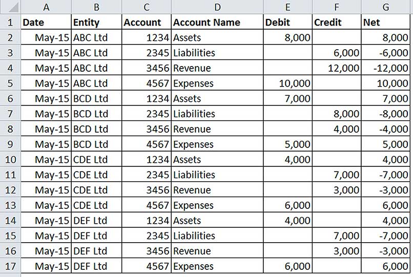
Figure 1 shows a simplified trial balance, with columns added for Date, Entity and Net. (Note: profit has not been transferred out.) Columns A, B and G have been added to the standard trial balance layout. Columns A and B have been entered manually, while column G has a simple formula =E2-F2 that has been copied down.
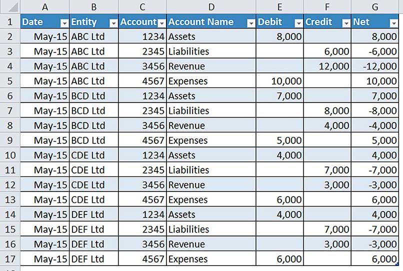
I highly recommend using the Format as Table icon situated in the middle of the Home ribbon tab. It is much more than just a formatting tool, as it adds extra functionality to the table. Format as Table was added in Excel 2007. Figure 2 shows the table after Format as Table has been applied.
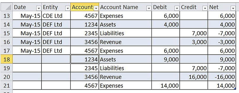
When you paste the next trial balance at the bottom of the table, the formula in column G (Net) is automatically copied down (as part of the Format as Table functionality). See Figure 3.
Figure 3 also shows that the column letters have been replaced by the column headings. This happens automatically and means you no longer need to use the Freeze Panes option to keep the headings visible as you scroll down the sheet. This is another built-in feature of Format as Table.
Once the consolidated data table is created you can then use either a PivotTable report or build a formula-based report to summarise and consolidate the trial balances.
Pivot table report
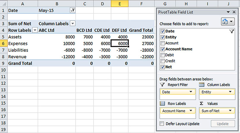
Figure 4 shows a simple PivotTable report summarising and consolidating the four entities. This is based on the data in Figure 2 (not Figure 3) and took less than 20 seconds to create.When the next month is added you simply refresh (Alt + F5) the PivotTable and then amend the filter in cell B1 to filter for the current month. The major advantage with PivotTable reports is that they automatically include any new codes in the data when refreshed.
However a problem with the PivotTable option is that layouts and formats are limited and often not board-presentation quality.
Formula-based report
With formula-based reports you can design the report from scratch and lay it out exactly as you want. The main function you use is SUMIFS. This function performs a multiple criteria sum. The SUMIFS function was added in Excel 2007.
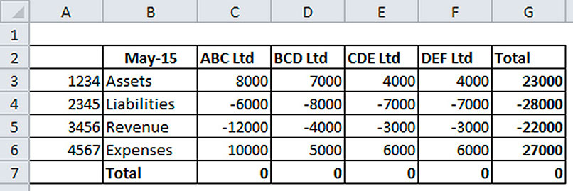
Figure 5 shows a formula-based report that replicates the PivotTable report. Row 7 and column G both have simple SUM functions adding up the detail. The trial balance table from Figure 2 is in a sheet called Data.
The formula in cell C3, that has been copied down and across is: =SUMIFS(Data!$G:$G,Data!$A:$A,$B$2,Data!$B:$B,C$2,Data!$C:$C,$A3)
This formula above is a three criteria SUMIFS. All three criteria must be met before the value in column G is summed. The $ signs ensure the references do not change as the formula is copied across and down.
Want to improve your Excel data management skills?
Consolidations
The above reports have ignored inter-company transactions. These would need to be handled as a separate process.
Syntax
SUMIFS(Range_to_Sum, Criteria_Range_1,Criteria_1, Criteria_Range_2,Criteria_2),…)
Range_to_Sum – The range that contains the values to be summed. In our example from Figure 2, column G is the Net column and that will be summed. These ranges are usually fixed references as shown in our example.
Criteria_Range_1 – the range that contains the first criteria. In our example this is the Date column, column A. These are usually fixed references. Criteria_1 – the entry to search for in Criteria_Range_1. In our case this is cell B2, which contains the date 1/5/15.
Criteria_Range_2 – the range that contains the second criteria. In our example this is the Entity column, column B. These are usually fixed references. Criteria_2 – the entry to search for in Criteria_Range_2. In our case this is cell C2, which contains an entity name.
Criteria_Range_3 – the range that contains the third criteria, which in our example is the Account Number column, column C. These are usually fixed references. Criteria_3 – the entry to search for in Criteria_Range_3. In our case this is cell A3, which contains the account number 1234.
More criteria can be specified by adding more ranges and criteria to the end of the function. The limit is 127 separate criteria.
The problem with formula-based reports is that they need to be maintained. If a new account code or entity is added, it must be inserted into the report. PivotTables handle that automatically each time they are refreshed.
A single data sheet is the goal. It makes creating reports so much easier, whether you use a PivotTable or a formula-based report.
Excel Tip
The keyboard shortcut to apply Format as Table is Ctrl + t. This uses the default colour settings. The colour and other table format settings can be changed in the Design ribbon tab.
Neale Blackwood CPA runs A4 Accounting, providing Excel training, webinars and consulting services to various organisations. Questions can be sent to [email protected]

