Loading component...
At a glance
Text boxes are independent of the Excel grid, and can be positioned anywhere on the sheet.
Text boxes can be used to:
- add instructions to specific areas of a sheet
- provide dynamic headings for reports
- insert large numbers for dashboards
- add detailed commentary to reports
You can format a text box to:
- remove its border so it looks better on a dashboard
- remove the fill colour and make it transparent
- create large, prominent numbers for dashboards
Linked text box
A text box can be linked to a cell. This means you can use formulas and functions in a cell to create a dynamic heading, sentence or calculation, and then have the freedom to place it anywhere on the sheet.
Linked text boxes have a limitation. You can only apply formats to the whole text box. Normal text boxes allow you to apply multiple formats to individual parts of the text.
Grouping text boxes
You can use grouping to combine multiple text boxes to get the best of both worlds.
Keyboard shortcut
You can insert a default text box in the middle of the sheet by pressing in sequence Alt N X. Don’t hold the keys down.
Worked example
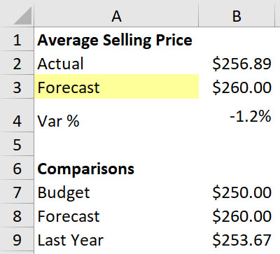
In Figure 01, we have the sheet structure that we will use to create a group of text boxes to display on a report or dashboard. There is a drop-down in cell A3 that allows you to choose a different comparison figure from the list below. The formulas are explained in the companion video to this article.
To insert a text box, click the Insert ribbon and click the Text Box icon on the far right.
Then use the mouse to draw the text box above the sheet grid.
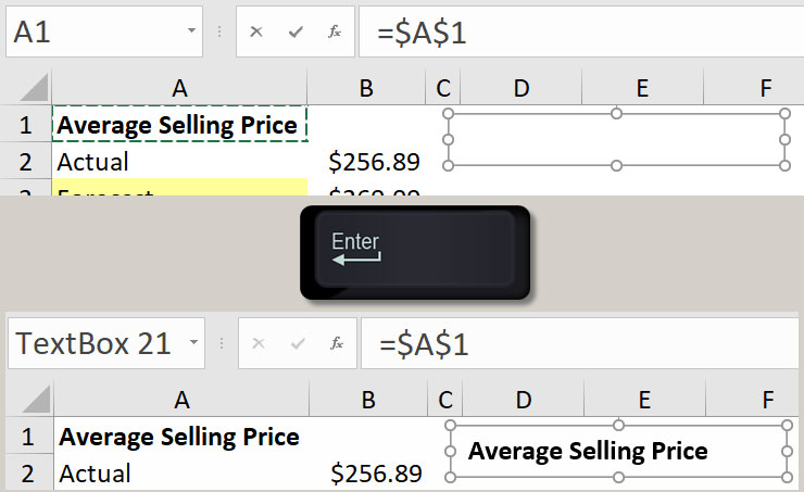
To link a text box to a cell, have the text box selected, click in the Formula Bar and press = and then click the cell to link to and press Enter – see Figure 02.
ou can apply multiple formats to the linked text box, but not to individual words within the linked text box. In Figure 03, I have centred the text horizontally and vertically and added a black fill plus a white font. You can use the Alignment and Font icons on the Home ribbon to achieve this. If you change the linked cell reference from one cell to another, it resets any font settings, and you need to redo them.

Using the same technique, I have added six more text boxes to contain headings and values – see Figure 04.
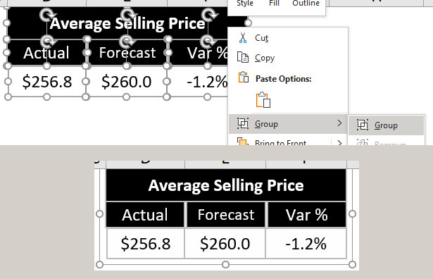
At the moment, these are seven separate text boxes. To easily position them on a dashboard or report, we need to group them together. You can hold the Ctrl key down and use the mouse to click on each text box. Be careful not to move the text boxes as you click them. Right-click on one of the selected text boxes and choose Group and Group – see Figure 05.
This converts seven separate text boxes into a single object that can be easily moved and positioned anywhere on the sheet.
Resizing tips
Resizing a text box can be fiddly. Here are some tips to make it easier.
Hold the Alt key down as you resize or move the text box. This “snaps to” the gridlines on the sheet beneath. This allows you to perfectly line up and resize text boxes. Hold the Shift key down to move a text box perfectly, horizontally or vertically.
Press the arrow keys when a shape is selected to move it perfectly, horizontally or vertically.
Copying and pasting a text box creates an exact copy of the size. This can be easier than starting a new text box.
When a text box is selected, a new Format ribbon tab is visible. This has options for alignment and grouping.
You can resize the grouped object, but the font sizes don’t scale. With the grouped object selected, you can reduce all the fonts using the Decrease Font Size icon on the Home ribbon.
Copying tip
If you want to copy or move a linked text box to another sheet, you need to include the sheet name in the formula.
There is a hack to do this without having to manually enter the sheet name. Create the text box as per normal. Click in the Formula Bar and press =, then use the mouse to go to another sheet and click a cell. Then return to the current sheet, click the correct cell and press Enter. The formula will now include the sheet name.
Linked pictures
This is a little-known Excel technique that comes with a warning. It can slow down the speed of your file. Use it sparingly. It can do amazing things, and you can combine it with text boxes.
Let’s say we want to tweak the example from earlier and we want to place a tick or a cross in the Variance % box if the variance is favourable or unfavourable.
We can use a conditional format to do that in cell B4, but it won’t be displayed in the text box.
I will demonstrate how to apply the conditional format in the companion video.
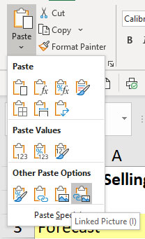
Once we have the desired cell entry, we can copy the cell and then click the large Paste drop-down on the Home ribbon (far left), and choose the Linked Picture icon (bottom-right icon) – see Figure 06.
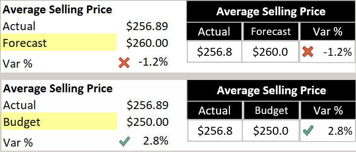
This pastes an exact copy of what the cell looks like, and allows you to resize it and treat it like a picture. Be warned: the resolution of the image when you increase the size isn’t perfect, as you can see from Figure 07.
Modifying the original cell will flow through to the linked picture, so be careful making changes to the cell. Depending on the changes you make, it may be easier to create a new picture.
Other shapes
Many of these techniques that work with text boxes also work with Excel’s shapes. Shapes are in the Insert ribbon, and can provide more variety than a standard text box. The shapes include Flowchart shapes if you need to create a flowchart for a process.
The companion video and Excel file will go into more detail to demonstrate these techniques.
Neale Blackwood CPA runs A4 Accounting, providing Excel training, webinars and consulting services to organisations around Australia. Questions can be sent to [email protected]

