Excel tips (advanced): how to use the slicer

Question

When I filter by more than one item in a PivotTable, it doesn’t display what those items are. Is there a way around this?

Answer

Filtering by multiple items in a PivotTable is best done with a Slicer. This is a graphic object that floats above the Excel grid. Slicers use buttons to allow you to select your filter items, and they display all the selected filter items. You need Excel 2010 or a later version to use Slicers.

Slicers only work with PivotTables in Excel 2010, and the ability to use Slicers with formatted tables was added in Excel 2013. A new addition in Excel 2013 is the Timeline Slicer, which handles date fields better than the standard Slicer.

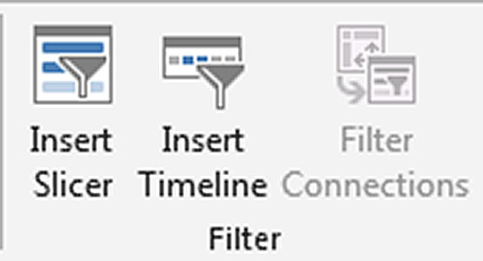
When a PivotTable is selected, click the Analyze ribbon tab. 

The Filter section has the Insert Slicer and Insert Timeline icons. 

See Figure 1. All screen shots are from Excel 2013. In Excel 2010, it is in the Options ribbon tab and the Sort & Filter section.

Just like a normal filter, you can select multiple fields (columns) to filter with a Slicer. Once created, the colours and sizing of the Slicer can be amended via the Options ribbon tab.

Slicers are filter controls and, as such, work in the same way as normal filters. The sequence in which you apply the filters will affect the other column filters. As a simple example, if you selected the state of WA, then all the postcodes displayed in a Postcode filter would start with 6, because all the other states’ postcodes would be filtered out.

I’m using a sample sales dataset for these examples. I have created a simple sales report based on state and product, and I will add a filter for customer category to the report.

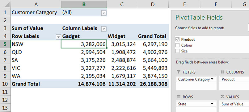
Example without a Slicer

Figure 2 shows the standard filter option for a PivotTable.

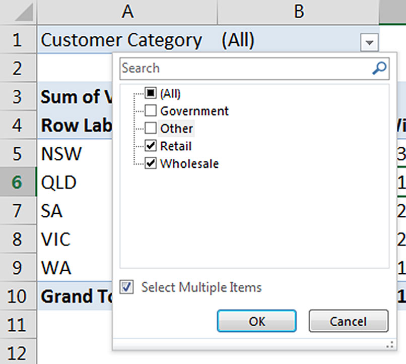
There is a drop down in cell B1 that allows you to choose the item(s) to filter by. There is an option to Select Multiple Items – see Figure 3

If you filter by multiple items, the PivotTable displays the (Multiple Items) message in the filter cell, which doesn’t communicate what filter has been applied – see Figure 4.

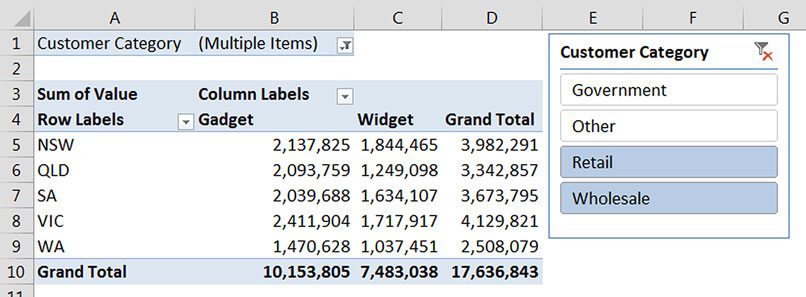
Example with a Slicer

If a filter is already in place when you add a Slicer, it will use the existing filter options when you insert it. If there is no filter in place when you add the Slicer, all the options will be selected. If I add the Slicer to the existing report, the filter items display immediately – see Figure 5.

To make a selection, you can click one of the buttons for a single item. To select multiple items, hold down the Ctrl key while clicking individual buttons.

You can also use the Shift key to select a group of buttons. Click the first button then hold the Shift key down and click the last button. This is handy for large lists of items. The icon in the top right corner of the Slicer clears the filter selections.

One thing a Slicer will allow that the standard filters won’t is including the filtered field in the report. Note that a field can’t be in the Filter section of a PivotTable and the Rows or Columns section. 

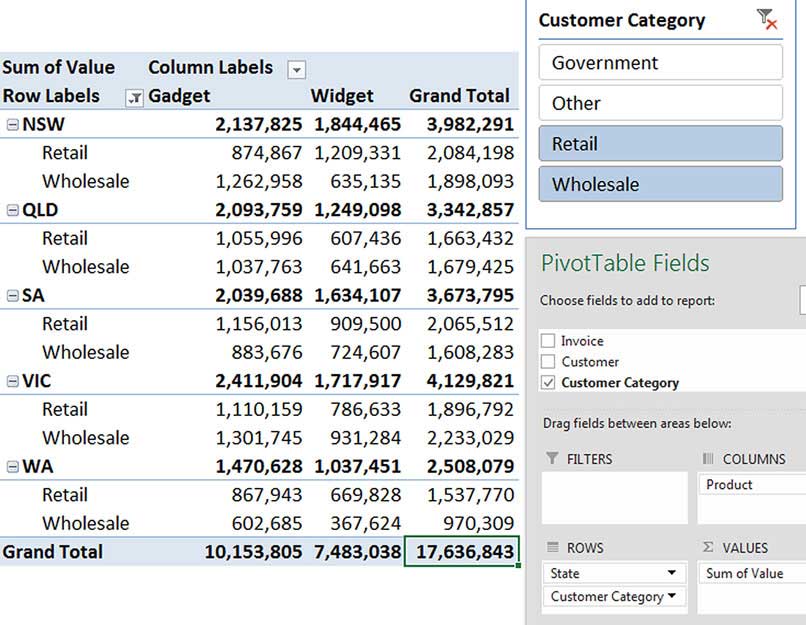
If a field is in the Filter section and you add it to the Rows section, it will disappear from the Filter section.

6 shows the Slicer field included in the report – I had to remove the customer category field from the Filter section, but the Slicer still works.

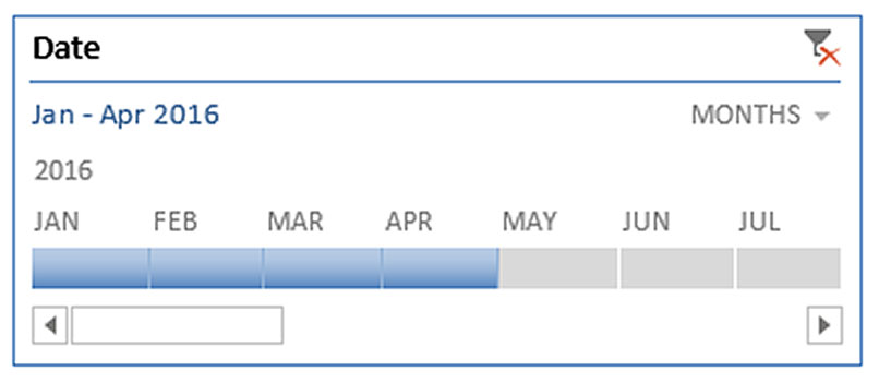
Timeline Slicer

Added in Excel 2013, the Timeline Slicer is designed to work only with date fields. When you insert a Timeline Slicer, it automatically identifies any date fields in the data and offers only them for selection. It handles months, quarters and years easily. An example of a Timeline Slicer for January to April 2016 is shown in Figure 7.

Controlling multiple PivotTables

Another advantage of using a Slicer is that it can control multiple PivotTables. For example, you might have different PivotTable reports that run off the same data source and you need to filter all the reports by the State field. You can control this with a single Slicer. Changing the State on the Slicer will filter all the PivotTable reports.

The downside of using a single Slicer to filter multiple PivotTables is that it is not obvious that the other PivotTables are filtered when the Slicer control is on another sheet. In this situation, it is worth adding a text box to the PivotTable report sheet explaining where the controlling Slicer is situated.

To control multiple PivotTables with a single Slicer, right click the Slicer and choose Report Connections. This will display a dialog listing each PivotTable and the sheet it is in. Tick the boxes of those you want to control. Note: only those PivotTables that use the same data source will be listed.

Slicers provide an easy-to-use interface to handle filtering for PivotTables and Formatted Tables. Try using them in your reports and dashboards to control PivotTable reports and PivotCharts.

The companion video and an Excel file may assist your understanding.

Neale Blackwood CPA runs A4 Accounting, providing Excel training, webinars and consulting services to organisations around Australia. Questions can be sent to [email protected]