Loading component...
At a glance
QUESTION
I need to display a numeric code with dashes between three sections, but I also need to be able to do calculations using the code. Is this possible?
ANSWER
Excel allows you to display numbers differently to the underlying value. You can use a custom number format to display the dashes while leaving the number itself unchanged.
Many codes have a structure built into them. Different sections of the code mean different things. You may need to increment a number in the middle of the code, which is difficult if you are using a text version of the code.
This technique applies to numeric codes only. If you are using an alphanumeric code you will have to use Excel’s text functions to manipulate it.
Worked example
If we take a seven-digit code that has three sections, separated by two dashes, we can see how to apply this technique.
1-23-4567
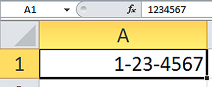
Figure 1 shows the underlying number of 1234567 in the formula bar of cell A1, while the number displayed on the grid contains the dashes.
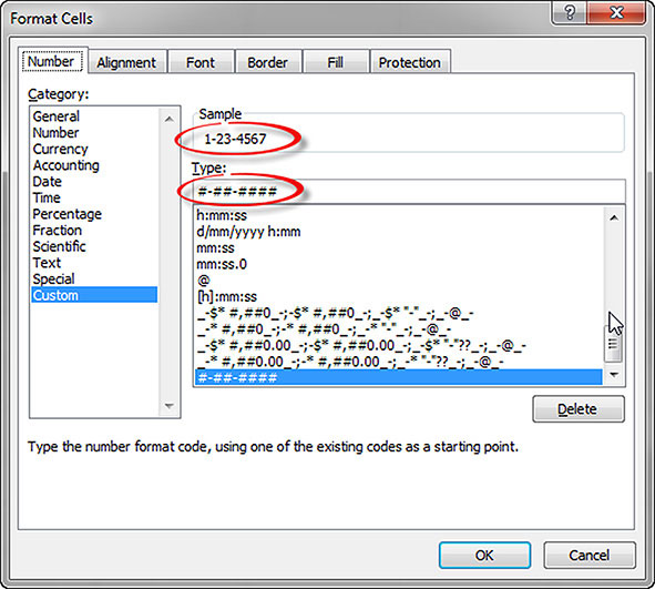
The format that achieves this is shown in Figure 2. You can press Ctrl + 1 to display the Format Cells dialog. As you create a custom number format in the Type box, Excel will display what the current cell’s contents with look like in the Sample section.
The format used is
#-##-####
The # symbol represents a numeric digit.
By using a custom number format to display the dashes in the number you can still use the underlying value in calculations.
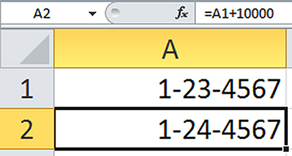
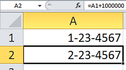
In our case we may want to increment that “23” section of the code by one. All we need to do is add 10,000 to the code as can be seen in cell A2 in Figure 3.
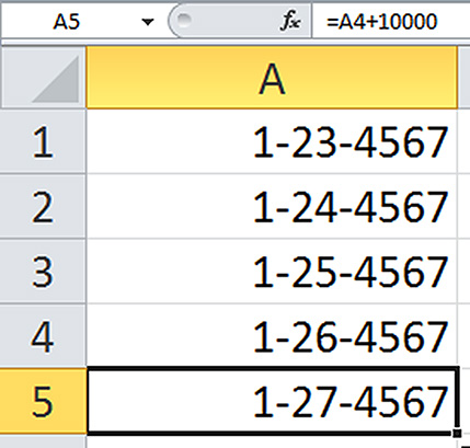
Copying this formula down would provide an easy way to increment the second section of the code without changing the other sections, as shown in Figure 4.
You will need to be careful in this case as you approach the 2 million value, as adding 10,000 will eventually increment the first digit of the code, which may not be what you require.
To increment the first digit just add 1,000,000 – see Figure 5.
Trailing characters
This technique can also be applied to displaying text characters after a number. For example, you may do calculations using metres and wish to display a value with a trailing m (for metre). But if you type the m after the value into a cell, it will be treated as text and Excel won’t perform any numeric calculations with the value. While the typical solution to this is to display the m in a separate column to the value, you could also use a custom number format to present the value with a trailing m.
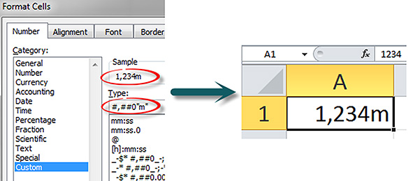
Figure 6 shows the custom number format used to display the m and the resulting cell format.
The custom number format used in Figure 6 is: #,##0”m”

Having the zero at the end of the hash symbols instructs Excel to display a zero numeral if there is a zero value, for example 0m. However, if you only use the hash characters to define the custom number format, Excel will not display a zero value. This means only the m will display, as can be seen in Figure 7.
Custom number formats provide many flexible options to display numbers and dates. The built-in custom number formats demonstrate many of these options and are worth reviewing.
Red brackets format
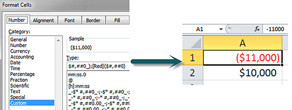
I am regularly asked how to display the red numerals and brackets for a negative number. Figure 8 has the answer. Note: the sample area in the Format Cells dialog won’t display any colours.
The custom number format used in Figure 8 is:
$#,##0_);[Red]($#,##0)
An unusual custom number format for a date is mmmmm. This will display J for a January date and D for December. It can be useful if you need to display a single character for a month when charting multiple months and when space is limited.
Neale Blackwood CPA runs A4 Accounting, providing Excel training, webinars and consulting services. Questions can be sent to [email protected]

