Excel tips: how to calculate dates and times

People will often struggle with date and time calculations in Excel, until they learn how it treats dates and times.

Dates – each date is a number. Excel’s calendar started on 1 January 1900. That was day 1. Each subsequent day has been allocated a sequential number. The number for 1 May 2018 is 43221. You don’t need to know the underlying number, but knowing that it is a numeral helps to explain how you can subtract one date from another to arrive at the number of days between the two dates. You are, in effect, subtracting one number from another.

Times – times are treated as fractions of a day. 0.5 is noon, 0.25 is 6am and 0.75 is 6pm. When dealing with times and durations such as hours and minutes, you are working with fractions (decimals).

Date and time formats

Another important concept to grasp with dates and times is that what is displayed in a cell is determined by the format applied to that cell. If you use the wrong format, then what is displayed can appear different to what is in the cell, and this can confuse users.

Sometimes when importing dates into Excel the dates are imported as dates and times. Hence, each date will include a fraction. If you are trying to perform calculations involving certain date ranges, this can affect the accuracy of the results.

A simple way to remove times (fractions) from dates is to use the TRUNC function, which truncates the number and removes the fraction – no rounding is done. In Figure 1, I have split the date/time in column A into the date and the time.

The formula in cell B2 is:
=TRUNC(A2)

The formula in cell C2 is:
 =A2-B2

Column B has been formatted as a date and column C as a time. Column C requires column B to calculate the time by subtracting the truncated date from the original date/time.

If you require a standalone formula to extract the time from a date/time you could use:
=A2-TRUNC(A2)

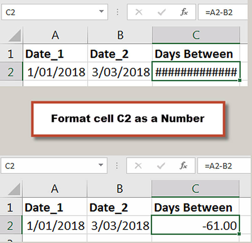
Subtracting one date from another will give the number of days between. When you subtract one date from another, Excel will typically format the formula cell as a date, too. You will need to change the cell format to a number. If the number is negative, Excel will display the # symbols as shown at the top of Figure 2.

Cell C2 has a simple =A2-B2 formula. Since it returns a negative, Excel displays the # symbols because a negative date is not possible. When you format the cell as a number, it works correctly as seen at the bottom of Figure 2.

Minutes

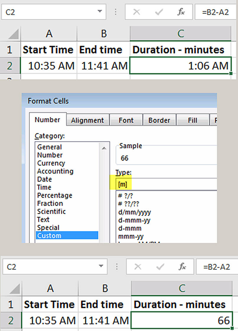
To display minutes correctly, you need to use a Custom Number Format. At the top of Figure 3, we deduct the start time from the end time and arrive at another time. This is 1 hour 6 minutes, but it is shown as a time, not a duration. To display the total minutes, you must use Custom Number Format [m]. The square brackets instruct Excel to exceed the normal 60-minute limit for minutes, so it displays 66 minutes (see bottom of Figure 3).

Hours

Excel limits the number of hours displayed to 24. If you add up a list of hours and it exceeds 24, only the remainder hours are shown (18:30), as on the left of Figure 4. To display the total number of hours, use Custom Number Format [h]:mm. The right side of Figure 4 shows the correct total hours.

Calculations with hours

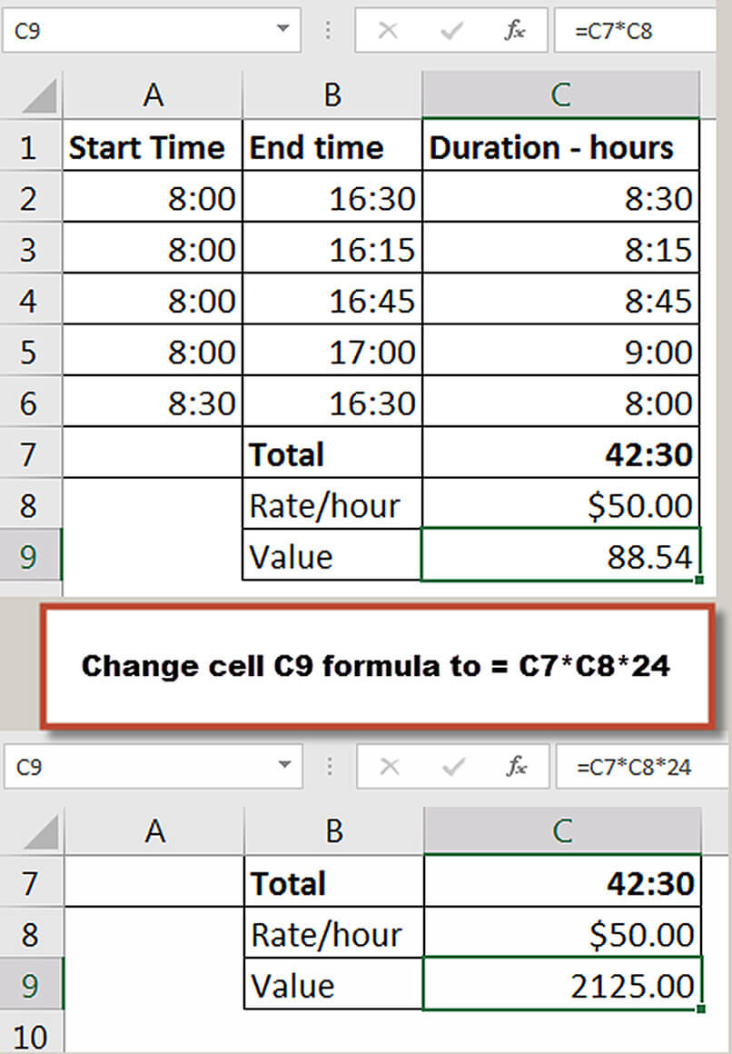
As mentioned before, what displays in a cell is based on the format of the cell. If we try to perform a calculation with cell C7 in Figure 4, we will run into an issue. If we multiply the 42:30 hours by $50, we end up with an incorrect number in cell C9 in the top section of Figure 5. Note: cell C9 has been formatted as a number.

The formula in cell C9 in the top section of Figure 5 is: =C7*C8. 

Because times are fractions of a day, to perform this type of calculation you will need to convert that fraction into hours. To do that, multiply the result by 24 as shown at the bottom of Figure 5, where Cell C9 contains =C7*C8*24.

Keyboard shortcuts

Two useful keyboard shortcuts for date and time entry are:
Ctrl + ; will insert the current date.
Ctrl + Shift + : will insert the current time in hours and minutes.

Current date 

There are two functions that calculate the current date. Both functions recalculate every time Excel calculates. Neither of these functions require an input between the parentheses.

NOW( ) – returns the current date and time. Note: this contains a fraction for the time.

TODAY( ) – returns the current date. This returns a whole number – no time included.

 

Working days

If you need to perform calculations involving working days, there are two functions worth exploring. Both automatically take weekends into account and holidays can also be specified.

WORKDAYS – adds a number of working days to a starting date.

NETWORKDAYS – returns the number of working days between two dates.

If you need more flexibility to handle different weekends (not all countries have a Saturday and Sunday weekend), you can use two functions added in Excel 2013, WORKDAYS.INTL and NETWORKDAYS.INTL. Both these have an extra option to allow you to specify the day(s) to treat as weekends.

The companion video and Excel file will go into more detail to demonstrate these techniques.

Neale Blackwood CPA runs A4 Accounting, providing Excel training, webinars and consulting services to organisations around Australia. Questions can be sent to [email protected]