At a glance

When creating budgets and forecasts you need to allocate amounts across months. I want to share a technique that simplifies allocating a value every one, two, three, four or six months.
The technique has a simple formula that uses a powerful but underused function called MOD. Figure 1 shows the structure we will use.
Columns A to D are used for input. For this allocation technique to work, the values in column D need to divide evenly into 12. Column E is what I call a helper column. This holds formulas that make the final formula shorter or simpler. The formula in column E simply divides the value from column C by the number of allocations in column D. This is the value that will be allocated in specific months.
Row 1 is a helper row. Our financial year doesn’t lend itself to easy monthly calculations, so I typically use a helper row with sequential month numbers to simplify calculations.
Note: all the formulas can be copied down and across. The formula in cell F3 is:
=IF(MOD(F$1,12/$D3)=0,$E3,0)
The IF function uses the MOD function as its logical test to determine whether or not to make an allocation in the month.
The MOD function returns the remainder after performing a division. In most cases this doesn’t appear to be a useful calculation but when used correctly it can simplify these types of calculations.
Within the MOD function 12 is divided by the number of allocations from column D. This represents the number of months between each allocation. Six allocations will result in an allocation every two months.
The MOD function divides the month number in row one by the number of months for the allocation and returns the remainder. When the remainder equals zero (the number of months divides evenly into the month number in row one) then the allocation will be made. In all other months zero will be returned. In the case of six allocations, the allocation will be made in every even month number.
As you can see from Figure 1, the value is allocated in the last month. If you need to have the allocation made in the first month then you need to adjust the formula slightly.
If you are making the change for every row, then the adjustment is simple. The amended formula for cell F3 is:
=IF(MOD(F$1,12/$D3)-1=0,$E3,0)
Deducting one from the result of the MOD function has the effect of putting the allocation in the first month, rather than the last month.

Figure 2 shows the amended formula in action.
The first formula worked in arrears with the allocation made in the last month, whereas the second formula works in advance and allocates the value in the first month. This means that July is allocated with all of the first entries.
You may want the ability to choose how to allocate on a row-by-row basis. In that case you need to modify the structure and the formula.

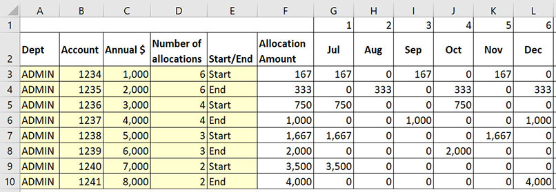
Figure 3 shows the amended structure. An extra column has been added to select whether to allocate at the start or the end of the period. We will use the entry in column E to determine whether to subtract one from the MOD function result.
The formula for cell G3 is:
=IF(MOD(G$1,12/$D3)-IF-($E3="Start",1,0)=0,$F3,0)
This replaces the -1 from the previous formula with an IF function. If column E contains the word Start then one is subtracted from the MOD function result. Otherwise zero is subtracted.
If you prefer shorter formulas, there is a formula that will return the same result. It uses a logic calculation instead of an IF function to return one or zero. The following formula will also work in cell G3:
=IF(MOD(G$1,12/$D3)-($E3="Start")=0,$F3,0)
This formula replaces the second IF function with a logical test. The logical test returns TRUE or FALSE. In Excel TRUE equals one and FALSE equals zero. To convert the TRUE and FALSE into their respective values you must enclose the logical test within parentheses (brackets). When the word Start is in column E, then the TRUE result will be converted into one and deducted from the MOD result. Otherwise a FALSE result is converted into zero and deducted.
This technique works well when you need to use a criteria to determine whether to perform a calculation or to display a zero value.
We can reduce the formula length even further by using only logical tests to perform the calculation. You can use logical tests in this manner if you are deciding between performing a calculation or displaying a zero. The shortest formula that I can create for cell G3 is:
=(MOD(G$1,12/$D3)-($E3="Start")=0)*$F3
The logical test that was used inside the IF function is used by itself enclosed in parentheses and that will return TRUE or FALSE. The result will be multiplied by the allocation amount in column F. When you multiply by TRUE you are in effect multiplying by one, so the value is unchanged. When you multiply by FALSE you are in effect multiplying by zero, which will return a zero.
The very first formula that we examined can also be rewritten in this way to create a shorter formula as below:
=(MOD(F$1,12/$D3)=0)*$E3
This technique works well when you need to use a criteria to determine whether to perform a calculation or to display a zero value.
My next article will demonstrate how to handle allocations that are not evenly spread throughout the year.
The companion video and Excel file will go into more detail to demonstrate these techniques.
Neale Blackwood CPA runs A4 Accounting, providing Excel training, webinars and consulting services to organisations around Australia. Questions can be sent to [email protected].

