Loading component...
At a glance
Adding checkboxes to Excel spreadsheets just got easier thanks to a recent update. You need the subscription version of Excel to access this new feature.
Checkboxes themselves are easy to use. In the past, it took a few steps to insert a checkbox and link it to a cell on the sheet. This process is now automated, and the results look much better than the old-fashioned Excel checkbox.
In Excel, checkboxes are typically used to turn calculations off and on. For example, costs in a budget may include an inflation component – you could use a checkbox to include or exclude the inflation component.
Checkboxes are either ticked or unticked. This means they can only return one of two results: a ticked checkbox returns TRUE; an unticked checkbox returns FALSE.
Both TRUE and FALSE are Excel keywords. If you type them in an Excel formula in lowercase they are always capitalised when the formula is complete.
TRUE and FALSE results are typically used as part of the first argument in an IF function. They can be used on their own in calculations which will be demonstrated later.
In Excel, TRUE equals one and FALSE equals zero. This means that if a cell containing TRUE is multiplied by a value, the value is unchanged. If a cell containing FALSE is multiplied by a value, it zeroes that value.
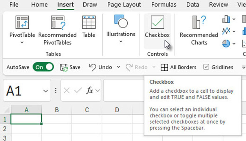
The Insert tab has a new option for Checkbox – see Figure 1. Checkboxes can be inserted into a single cell or a range of cells in one click.
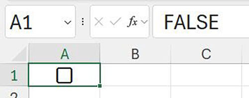
When a checkbox is inserted in a cell it is automatically linked to the cell. The new checkbox is unticked, and the cell contains the word FALSE. The cell appears empty apart from the checkbox – see Figure 2.
As noted in the tool tip in Figure 1, you can select single or multiple checkbox cells and change them by pressing the spacebar.
If you delete the entry in the cell, you also delete the checkbox. This could cause issues as users may inadvertently delete a checkbox that is used as part of a calculation. The companion video suggests a solution.
Here are two examples using checkboxes.
Budget example
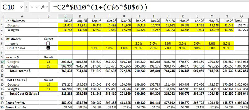
Figure 3 has a simple budget with income and cost of sales. There is a separate inflation rate for each. We need the ability to independently turn off the inflation calculations for income and cost of sales.
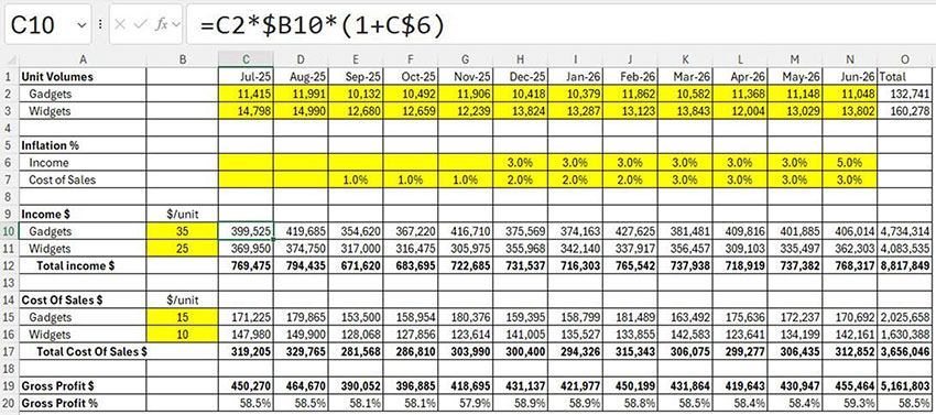
Input cells are yellow. The formula in cell C10 is:
=C2*$B10*(1+C$6)
The formula in cell C15 is:
=C2*$B15*(1+C$7)
These formulas have been copied down and across to populate the relevant range.
It is a simple process to convert these two formulas to use the checkbox cells to control each inflation calculation.
In Figure 4, two checkboxes have been added to the sheet and the formulas updated.
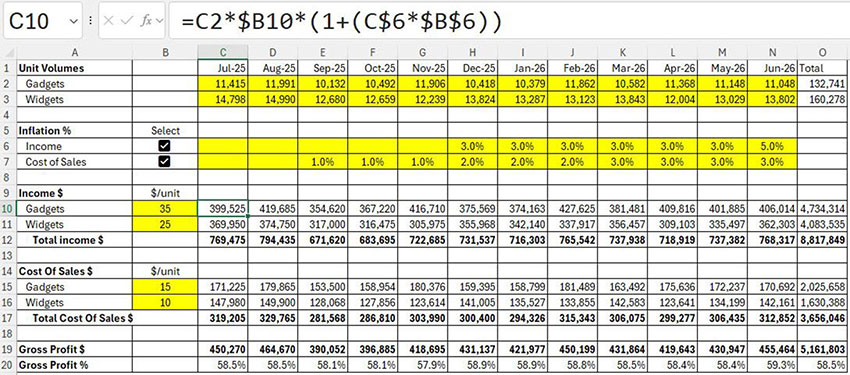
Remember a ticked checkbox cell contains TRUE and TRUE equals one. An unticked checkbox cell has FALSE and FALSE equals zero.
The revised formulas are shown below.
Cell C10:
=C2*$B10*(1+(C$6*$B$6))
Cell C15:
=C2*$B15*(1+(C$7*$B$7))
These formulas have been copied across and down to populate their respective ranges.
Changing (1+C$6) to (1+(C$6*$B$6)) zeroes the inflation component if cell B6 is FALSE (unticked). If cell B6 is TRUE (ticked), the inflation calculation is unchanged.
You can see the checkboxes in action in Figure 5 and Figure 6.

Alternative formulas
Below are the IF function versions of the two formulas. These can be copied across and down to populate the ranges.
Cell C10:
=C2*$B10*(1+IF($B$6,C$6,0))
Cell C15:
=C2*$B15*(1+IF($B$7,C$7,0))
To-do list example
Putting a line through a task on your to-do list can provide a lot of satisfaction. Excel can provide that feeling by combining checkboxes, a list and a conditional format.
Excel has a strikethrough format that puts a line through the text in a cell. We can use a conditional format to apply the strikethrough format to an entry in a list based on a checkbox.
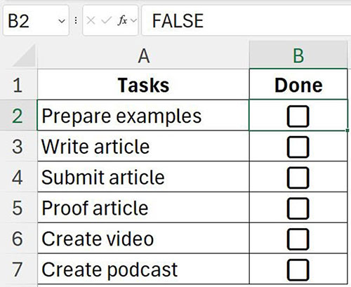
In Figure 7, there is a list of tasks with checkboxes already inserted next to them.
Here are the steps to apply a conditional format based on checkboxes.
1. Select the range A2:A7.
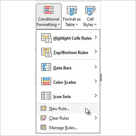
2. On the Home ribbon click the Conditional Formatting icon drop down and select New Rule – see Figure 8.
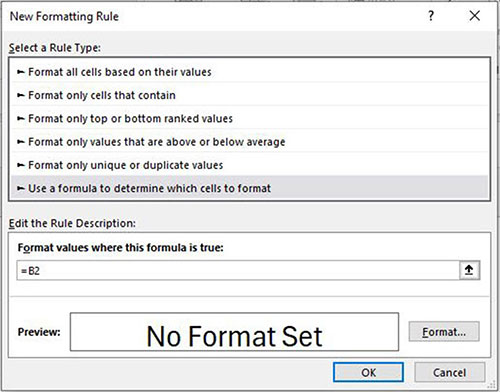
3. Select the last option in the top section “use a formula …”. See Figure 9.
4. Click in the box under the text “Format values where…” and type =B2. Make sure there are no $ signs in the formula. See Figure 9.
The formula you create in the box must return TRUE to apply a format. Because the checkbox cells display TRUE or FALSE, just referring to the checkbox cell is enough to control the conditional format.
When creating a formula for a conditional format for a range you must create the formula so that it applies to the top left cell of the range. In this case, it refers to cell B2 because the range starts in cell A2. The relative reference will apply correctly to all the other cells in the range A2:A7.
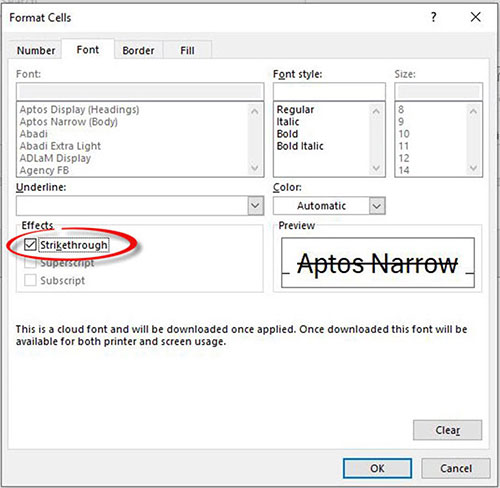
5. Click the Format button and on the Font tab tick the Strikethrough checkbox – see Figure 10.
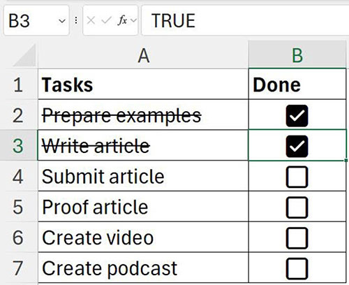
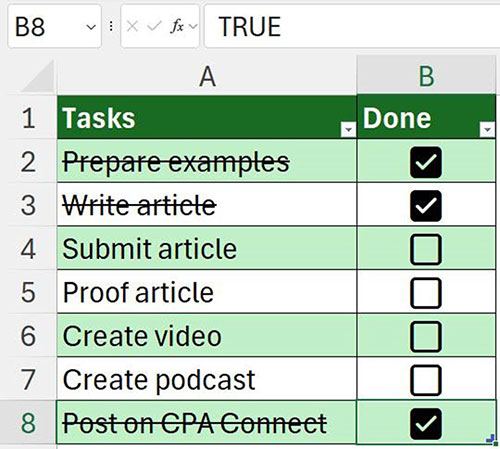
6. Click OK and OK again to apply the conditional format. See Figure 11 for the highly satisfying strikethrough format.
Formatted tables
The checkbox feature works in formatted tables. If checkboxes are in each cell in a column in a formatted table, then when you add another row to the table a new checkbox is automatically entered in the new row.
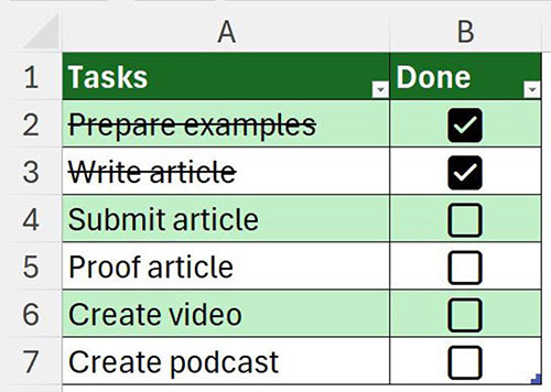
The to-do list has been converted into a formatted table in Figure 12.
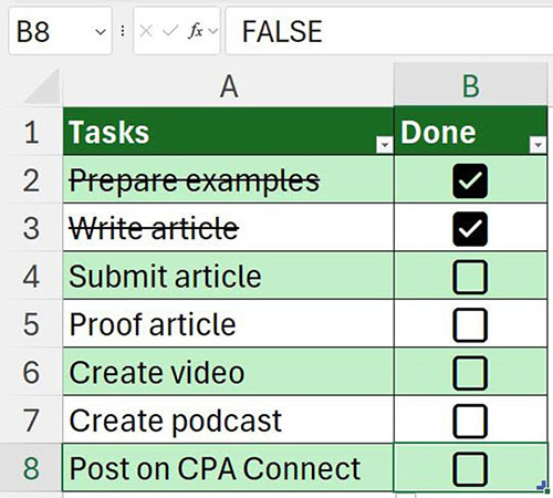
When a new task is added to the bottom of the list, an unticked check box is added (Figure 13) and the conditional format is also copied down to the new row (Figure 14).
Compatibility
If you send a file with the new checkboxes to someone who doesn’t have the checkbox feature, the checkboxes won’t display, and the checkbox cells will display TRUE or FALSE. Any formulas will still work. If they edit and save the file, the checkboxes should still be present when you open the file.
Checkboxes are an easy-to-use interface and now they are much easier to add and use in your spreadsheets.