Excel tips: how to solve tricky challenges using LET

I recently received an interesting query from a reader who created a list of departments and full-time equivalent (FTE) values using the UNIQUE function and the SUMIFS function and wanted the final report sorted in descending order based on the FTE numbers, without using any helper cells.

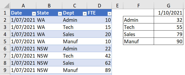
The reader tried using the SORT function on the Department column (created using the UNIQUE function), but that only sorted the department in alphabetical order. The snapshot of data and the current report structure are shown in Figure 1, using a formatted table in columns A to D, named tblFTE.

The formulas for the three cells in Figure 1 are listed and explained in Table 1.

I initially wanted to use the new SORTBY function, which sorts one column based on entries in another column. However, that created a circular reference between the FTE column and the Department column. The problem is that column F and column G have two separate formulas, with column G, which I needed to sort, linking back to column F.

Figure 2 shows the progression of formulas I used to arrive at the solution to this problem, without the use of helper cells. I recreated the existing report using LET and then managed to combine the two separate formulas into one table. The solution formula is in cell P2.

Table 2 lists the four formulas involved. These are all dynamic array formulas that spill based on their size. I will explain and discuss them below.

The first two formulas in Table 2 are the building blocks of the solution.

Cell I2 recreates the cell F2 formula using a LET function. The variable u holds the list of unique departments. Having the variable u as the last argument allows you to list all the entries in the variable. This technique is repeated in the formulas that follow.

Cell K2 recreates the cell G2 formula using a LET function. The variable v holds the summed values associated with each unique department held in variable u. Note that the SUMIFS uses the u variable as its last argument.

Cell M2 creates a table that matches the original report. The CHOOSE function combines the two variables u and v into a single table, held in the variable t.

Choose function

This function offers an alternative to multiple IF functions and works in a sequential manner best explained with some examples.

The first argument of CHOOSE is a whole number. The remaining arguments are a sequential list of entries separated by commas. One of these will be returned based on the number in the first argument.

=CHOOSE(3,"First","Second","Third")

This formula returns the text Third. If the first argument in the CHOOSE were 4, this formula would return an error, because there are only three arguments after the first argument.

Assume cell A1 contains the date 1/7/2021.

=CHOOSE(MONTH(A1),3,3,3,4,4,4,1,1,1,2,2,2)

This formula will return 1, which is the seventh argument after the first argument.

The MONTH function returns the calendar month, 7 in this case. The above CHOOSE function converts the calendar month number (7) from cell A1 into the Financial Year quarter number (1).

Choose magic

We can use array syntax in the first argument to combine entries. Array syntax has entries separated by commas between braces (curly brackets). Array syntax allows you to use more than one value as the first argument. When used as the first argument in the CHOOSE function, array syntax can create a table structure. See example below in Figure 3. 

=CHOOSE({1,2,3,2},"First","Second","Third") 

This formula creates a horizontal list of four entries based on the four numbers between the braces.

Used by itself, this formula spills across the columns to the right.

We used the following CHOOSE function as part of the solution.

CHOOSE({1,2},u,v)

This creates a table with the unique department codes (u) in the first column and the corresponding summed values (v) in the second column. We captured this table in the t variable. This solves the problem we had in columns F and G, where we had two separate lists.

In cell M2 I have displayed the virtual table held in the t variable. We now have a two-column table that we can use with the SORT function.

In the final formula in cell P2, we take this table (t) and sort it by the second column (2) and in descending order (-1). 

SORT(t,2,-1)

LET function recommended display

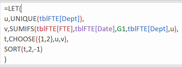
When creating long LET functions like these, it can be helpful to display the formula as shown in Figure 4.

This defines the variables on separate lines at the top of the formula, and the output is the last entry.

To enter the line breaks in the Formula Bar, use Alt + Enter.

This example shows how powerful Excel’s dynamic array functions are and how useful the LET and CHOOSE functions can be in solving difficult problems and avoiding circular references.

Things to note

• By using a formatted table as the data source, you automatically include any new rows added in the calculation.
• The MAX function in cell G1 extracts the latest date from the data.
• The UNIQUE function identifies any new departments in the data and lists them.
• The CHOOSE function combines lists together to create a table.
• The SORT function updates automatically based on the latest values

The companion video and Excel file will go into more detail to demonstrate these techniques.

Neale Blackwood CPA runs A4 Accounting, providing Excel training, webinars and consulting services. Questions can be sent to [email protected]